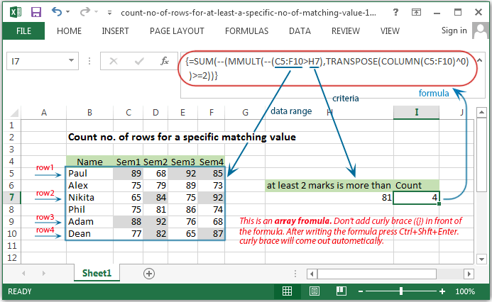
Excel Formulas - Count number of rows for a specific matching value

Count number of rows for a specific matching value

Syntax of used function(s)

SUM(range)
MMULT(array1, array2)
COLUMN([reference])
TRANSPOSE(array)

The SUM function, one of the math and trig functions, adds values.
The MMULT function returns the matrix product of two arrays. The result is an array with the same number of rows as array1 and the same number of columns as array2.
The COLUMN function returns the column number of the given cell reference.
The TRANSPOSE function returns a vertical range of cells as a horizontal range, or vice versa.

What to do?

To count rows that contain atleast a specific number of matching values, the array formula based on the MMULT, TRANSPOSE, COLUMN, and SUM functions can be used. In the example shown, the formula in G7 is:

{=SUM(--(MMULT(--(C5:F10>H7),TRANSPOSE(COLUMN(C5:F10)^0))>=2))}

The above formula is an array formula, it must be used ctrl+shift+enter key.

Formula

=SUM(--(MMULT(--(C5:F10>H7),TRANSPOSE(COLUMN(C5:F10)^0))>=2))

How this formula works

Inside the above formula the logical criteria used is:

--(C5:F10>H7)

This formula generates a TRUE and FALSE result for every value in the range C5:F10 and the double negative (--) converts it into 1 and 0 and the array looks like

{1;0;1;1; 0;0;1;0; 0;1;0;1; 0;0;1;0; 1;1;0;0; 0;1;0;1;}

This array formed by 6 rows and 4 columns (6x4) and go for next execution to MMULT function as array1 and the array2 is created from

TRANSPOSE(COLUMN(C5:F10)))

The COLUMN function is used to generate a numeric array of the right size. Therefore the matrix multiplication with MMULT funcntion done.
The column count in array1 (4) must equal the row count in array2.

COLUMN returns the 4-column array {3,4,5,6}, and TRANSPOSE changes this array to the the 4-row array {3;4;5;6;}. MMULT then runs and returns a 6 x 1 array result looks like -

{14;0;10;0;7;10}

Therefore check for non-zero entries with >2 and again convert the TRUE FALSE to 1 and 0 with a double negative and the array looks like -

{1;0;1;0;1;1;}

And finally the SUM function add the array and returns result.

Previous: Excel Formulas - Count number of cells containing any text
Next: Excel Formulas - Count rows matching two criterias in two columns within a row