Generate a 3D dataset and perform multidimensional scaling (MDS) using SciPy

NumPy: Integration with SciPy Exercise-9 with Solution

Write a Numpy program to generate a 3D dataset and perform multidimensional scaling (MDS) using SciPy.

Sample Solution:

Python Code:

import numpy as np  # Import NumPy library
from scipy.spatial.distance import pdist, squareform  # Import pdist and squareform for distance calculation
from sklearn.manifold import MDS  # Import MDS from scikit-learn for multidimensional scaling
import matplotlib.pyplot as plt  # Import matplotlib for plotting

# Generate a 3D dataset with 10 points
np.random.seed(0)  # Seed for reproducibility
data_3d = np.random.rand(10, 3)

# Compute the distance matrix
dist_matrix = squareform(pdist(data_3d, 'euclidean'))

# Perform Multidimensional Scaling (MDS)
mds = MDS(n_components=2, dissimilarity='precomputed', random_state=0)
data_2d = mds.fit_transform(dist_matrix)

# Print the original 3D data and the transformed 2D data
print("Original 3D Dataset:")
print(data_3d)

print("\nTransformed 2D Dataset using MDS:")
print(data_2d)

# Plot the original 3D dataset
fig = plt.figure()
ax = fig.add_subplot(121, projection='3d')
ax.scatter(data_3d[:, 0], data_3d[:, 1], data_3d[:, 2], c='r', marker='o')
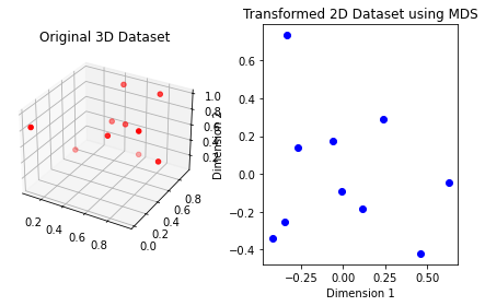
ax.set_title('Original 3D Dataset')

# Plot the transformed 2D dataset
plt.subplot(122)
plt.scatter(data_2d[:, 0], data_2d[:, 1], c='b', marker='o')
plt.title('Transformed 2D Dataset using MDS')
plt.xlabel('Dimension 1')
plt.ylabel('Dimension 2')

# Show the plots
plt.tight_layout()
plt.show()

Output:

Original 3D Dataset:
[[0.5488135  0.71518937 0.60276338]
 [0.54488318 0.4236548  0.64589411]
 [0.43758721 0.891773   0.96366276]
 [0.38344152 0.79172504 0.52889492]
 [0.56804456 0.92559664 0.07103606]
 [0.0871293  0.0202184  0.83261985]
 [0.77815675 0.87001215 0.97861834]
 [0.79915856 0.46147936 0.78052918]
 [0.11827443 0.63992102 0.14335329]
 [0.94466892 0.52184832 0.41466194]]

Transformed 2D Dataset using MDS:
[[-0.00549785 -0.09249204]
 [-0.05957237  0.17530568]
 [-0.34750737 -0.25221217]
 [ 0.11576864 -0.18536257]
 [ 0.4561849  -0.41964991]
 [-0.33109392  0.73362778]
 [-0.42005493 -0.34160784]
 [-0.26778615  0.1395934 ]
 [ 0.62383177 -0.04708346]
 [ 0.23572727  0.28988113]]

Explanation:

• Import Libraries:
• Import the necessary libraries: NumPy for array creation and manipulation, SciPy for distance calculations, scikit-learn for Multidimensional Scaling (MDS), and matplotlib for plotting.
• Generate 3D Dataset:
• Generate a 3D dataset with 10 points using "np.random.rand()". Seed the random number generator for reproducibility.
• Compute Distance Matrix:
• Compute the pairwise Euclidean distance matrix using pdist and squareform from SciPy.
• Perform Multidimensional Scaling (MDS):
• Use MDS from scikit-learn to transform the distance matrix into a 2D dataset. Set n_components to 2 to reduce the dimensionality to 2D and dissimilarity to 'precomputed' to use the precomputed distance matrix.
• Print Results:
• Print the original 3D dataset and the transformed 2D dataset to verify the transformation.
• Plot the Original and Transformed Datasets:
• Plot the original 3D dataset using a 3D scatter plot and the transformed 2D dataset using a 2D scatter plot with matplotlib.
• Finally display the plots using plt.show().

Python-Numpy Code Editor:

Have another way to solve this solution? Contribute your code (and comments) through Disqus.

Previous: Ordinary differential equations with NumPy and SciPy.
Next: Create and operate on a large Sparse matrix using SciPy's Sparse module.