Mastering np.polyfit for Curve fitting in Python

Comprehensive Guide to np.polyfit in Python

np.polyfit is a NumPy function used to fit a polynomial of a specified degree to a set of data points using the least squares method. It is widely used in data analysis, curve fitting, and mathematical modeling. The function returns the coefficients of the polynomial that best fits the data.

Syntax:

numpy.polyfit(x, y, deg, rcond=None, full=False, w=None, cov=False)

Parameters:

• x (array-like): 1-D array of x-coordinates of the data points.
• y (array-like): 1-D array of y-coordinates of the data points.
• deg (int): Degree of the fitting polynomial.
• rcond (float, optional): Relative condition number for filtering singular values. Default is len(x) * eps.
• full (bool, optional): If True, returns additional diagnostic information.
• w (array-like, optional): Weights for the y-coordinates of the data points.
• cov (bool, optional): If True, returns the covariance matrix of the polynomial coefficients.

Returns:

• p (ndarray): Polynomial coefficients in descending powers.
• others (optional): Diagnostic information, residuals, rank, singular values, or covariance matrix (if requested).

Examples:

Example 1: Fit a Linear Polynomial

Code:

import numpy as np

# Define data points
x = np.array([0, 1, 2, 3, 4])
y = np.array([1, 3, 7, 13, 21])

# Fit a linear polynomial (degree = 1)
coefficients = np.polyfit(x, y, deg=1)

# Print the coefficients
print("Linear polynomial coefficients:", coefficients)

Output:

Linear polynomial coefficients: [ 5. -1.]

Explanation:

This example fits a line (y = mx + c) to the data points. The returned coefficients represent the slope (m) and intercept (c).

Example 2: Fit a Quadratic Polynomial

Code:

import numpy as np

# Define data points
x = np.array([-2, -1, 0, 1, 2])
y = np.array([4, 1, 0, 1, 4])

# Fit a quadratic polynomial (degree = 2)
coefficients = np.polyfit(x, y, deg=2)

# Print the coefficients
print("Quadratic polynomial coefficients:", coefficients)

Output:

Quadratic polynomial coefficients: [ 1.00000000e+00 -2.21509051e-16  0.00000000e+00]

Explanation:

A second-degree polynomial (y = ax^2 + bx + c) is fitted to the data. The coefficients correspond to the terms in descending powers.

Example 3: Use the Polynomial for Predictions

Code:

import numpy as np

# Define data points
x = np.array([0, 1, 2, 3, 4])
y = np.array([1, 3, 7, 13, 21])

# Fit a linear polynomial
coefficients = np.polyfit(x, y, deg=1)

# Create a polynomial function
polynomial = np.poly1d(coefficients)

# Predict values for new x values
x_new = np.array([5, 6, 7])
y_new = polynomial(x_new)

# Print predictions
print("Predicted y values for x = [5, 6, 7]:", y_new)

Output:

Predicted y values for x = [5, 6, 7]: [24. 29. 34.]

Explanation:

np.poly1d creates a polynomial function from the coefficients, which can be used for predictions or further computations.

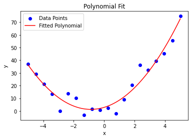
Example 4: Visualize Polynomial Fit

Code:

import numpy as np
import matplotlib.pyplot as plt

# Define noisy data points
x = np.linspace(-5, 5, 20)
y = 2 * x**2 + 3 * x + 5 + np.random.normal(scale=5, size=x.shape)

# Fit a quadratic polynomial
coefficients = np.polyfit(x, y, deg=2)

# Create the polynomial function
polynomial = np.poly1d(coefficients)

# Generate smooth x values for plotting
x_smooth = np.linspace(-5, 5, 100)
y_smooth = polynomial(x_smooth)

# Plot the data and the fit
plt.scatter(x, y, label="Data Points", color="blue")
plt.plot(x_smooth, y_smooth, label="Fitted Polynomial", color="red")
plt.title("Polynomial Fit")
plt.xlabel("x")
plt.ylabel("y")
plt.legend()
plt.show()

Output:

Explanation:

This example demonstrates how to visualize the polynomial fit alongside noisy data points.

Example 5: Extract Residuals and Diagnostics

Code:

import numpy as np

# Define data points
x = np.array([0, 1, 2, 3, 4])
y = np.array([1, 3, 7, 13, 21])

# Fit a linear polynomial and get diagnostics
coefficients, residuals, rank, singular_values, rcond = np.polyfit(x, y, deg=1, full=True)

# Print diagnostics
print("Residuals:", residuals)
print("Rank of matrix:", rank)
print("Singular values:", singular_values)
print("Relative condition number:", rcond)

Output:

Residuals: [14.]
Rank of matrix: 2
Singular values: [1.34777468 0.42837299]
Relative condition number: 1.1102230246251565e-15

Explanation:

The full=True option provides detailed diagnostic information about the fitting process, including residuals and the rank of the matrix.

Additional Notes:

1. Applications: Curve fitting, trend analysis, and mathematical modeling.

2. Precision Control: Adjust the deg parameter to control the complexity of the fit.

3. Covariance Matrix: Use cov=True to understand the reliability of the coefficients.

Practical Guides to NumPy Snippets and Examples.